Introduction to Singular Learning Theory
2026-10-15 Iliad Intensive

Statistical Learning

Relative Information

  • Given probability distributions \(q\) and \(p\) on a finite set \(X\), the relative information (Kullback-Leibler divergence, relative entropy) from \(p\) to \(q\) is \[ I_{q\Vert p}(X) = \sum_{x\in X} q(x) \log \frac{q(x)}{p(x)}. \]
  • Given probability densities \(q\) and \(p\) on an infinite set \(X\), the relative information is \[ I_{q\Vert p}(X) = \int q(x) \log \frac{q(x)}{p(x)}\, dx. \]
  • Well-defined iff \(p(x)=0\) implies \(q(x) = 0\) for all \(x\) (absolute continuity \(q \ll p\)).
  • Think of this as the distance of a model distribution \(p\) to the true distribution \(q\). This distance is not symmetric, i.e. \(I_{q\Vert p}(X) \neq I_{p\Vert q}(X).\)

Maximum Likelihood

  • Let \(p(x|\omega)\) be the model likelihood of data \(x\) given parameters \(\omega \in \Omega\).
  • Suppose we observe data \(x_{[n]} = (x_1, \ldots, x_n) \in X^n\).
  • Loss (normalized negative log-likelihood) \(L_n(\omega) = -\frac{1}{n}\sum_{i} \log p(x_i|\omega)\).
  • Maximum likelihood estimate \(\hat{\omega} = \operatorname*{arg\,min}_{\omega} L_n(\omega)\).
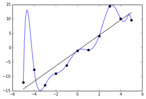
  • Problem. Overfitting the data. Perhaps we have been doing it wrong.
Stochastic Gradient Descent

  • Instead, suppose we could minimize the relative information (despite not knowing \(q\)). \[ I(\omega) := I_{q\Vert p(\cdot\vert\omega)}(X) = \int q(x) \log \frac{q(x)}{p(x|\omega)}\, dx \]
  • Optimize using gradient descent with \[ \frac{dI}{d\omega}(\omega) = - \int q(x) \frac{\partial}{\partial\omega} \log p(x|\omega)\, dx. \]
  • Estimate the gradient by sampling \(x\) from \(q\) (or data \(x_{[n]}\)). Note similarity to \[\frac{dL_n}{d\omega}(\omega) = -\frac{1}{n}\sum_i \frac{d}{d\omega} \log p(x_i|\omega).\]
  • Advantage. Popular technique in deep learning. Tends to overfit less. Regularization.

Bayesian Inference

  • Initially, let the prior on model parameters be \(p(\omega)\).
  • We update our prior to the posterior \[ p(\omega|x_{[n]}) = \frac{p(x_{[n]}|\omega)p(\omega) }{p(x_{[n]})} = \frac{p(x_{[n]}|\omega)p(\omega) }{\int p(x_{[n]}|\omega)p(\omega)\, d\omega}. \]
  • We infer new data points using the predictive distribution \[ p^*(x) := p(x|x_{[n]}) = \int p(x|\omega)p(\omega|x_{[n]})\, d\omega. \]
  • These integrals are difficult to compute or even estimate!

Model Selection

  • Which model \(M_1, \ldots, M_m\) best describes the data \(x_{[n]}\)?
  • Assign priors \(p(M_j)\) and \(p(\omega|M_j)\), and compute \[ p(M_j|x_{[n]}) \propto p(x_{[n]}|M_j)\, p(M_j) \] where \(Z_n(M_j) = p(x_{[n]}|M_j)\) is the marginal likelihood \[ Z_n(M_j) = \int_\Omega e^{-n L_n(\omega \vert M_j)}\, p(\omega|M_j)\,d\omega. \]
  • The free energy or stochastic complexity is \(F_n(M_j) = -\log Z_n(M_j)\).
  • Select the model with the smallest free energy.

Likelihood and Relative Information

empirical expectation
loss (negative log-likelihood) \(L_n(\omega) = -\frac{1}{n}\sum_i \log p(x_i\vert\omega)\) cross-entropy
\(L(\omega) = \mathbb{E}[L_n(\omega)]\)
empirical entropy
\(S_n = -\frac{1}{n}\sum_i \log q(x_i)\)
entropy
\(S = \mathbb{E}[S_n]\)
log-likelihood ratio \(I_n(\omega) = \frac{1}{n}\sum_i \log \frac{q(x_i)}{p(x_i\vert\omega)}\) relative information
\(I(\omega) = \mathbb{E}[I_n(\omega)]\)
relationship
\(L_n(\omega) = S_n + I_n(\omega)\)
relationship
\(L(\omega) = S + I(\omega)\)

Free Energy and Relative Information

empirical expectation
free energy \(F_n = -\log \int_\Omega e^{-n L_n(\omega)}\, p(\omega)\, d\omega = -\log p(x_{[n]})\) cross-entropy
\(F = \mathbb{E}[F_n]\)
normalized free energy \(F^0_n = -\log \int_\Omega e^{-n I_n(\omega)}\, p(\omega)\, d\omega = \log \frac{q(x_{[n]})}{p(x_{[n]})}\) relative information
\(I_{q\Vert p}(X^n) = \mathbb{E}[F^0_n]\)
relationship
\(F_n = n S_n + F^0_n\)
relationship
\(F = n S + I_{q\Vert p}(X^n)\)

Bayesian Information Criterion

  • The (empirical) Fisher information matrix is the Hessian of the loss, or equivalently of the log-likelihood ratio, since \(S_n\) does not depend on \(\omega\): \[ J_n(\omega) = \partial^2 L_n(\omega) = \partial^2 I_n(\omega). \]
  • A model is regular if it is identifiable (\(\omega \mapsto p(\cdot|\omega)\) is one-to-one) and its Fisher information matrix \(J(\omega) = \mathbb{E}_{x_{[n]} \sim p(\cdot|\omega)}\big[J_n(\omega)\big]\) is invertible for all \(\omega\).
  • Laplace approximation. Suppose the model is regular, with \(\dim \Omega = d\). If the loss \(L_n(\omega)\) is uniquely minimized at the MLE \(\hat{\omega}\) and \(J_n(\hat{\omega})\) is full rank, then as \(n \rightarrow \infty\), \[ F_n \approx n L_n(\hat{\omega}) + \frac{d}{2} \log n + O_p(1). \]
  • Bayesian information criterion (BIC): select the model minimizing \(n L_n(\hat{\omega}) + \frac{d}{2} \log n\).
  • Tradeoff between accuracy (fit to data) and complexity (number of parameters).

Legendre Duality

  • The log-partition function \(\Lambda(f) = \log \int_\Omega e^{f}\, p\, d\omega\) and relative information \(q \mapsto I_{q\Vert p}(\Omega)\) are Legendre duals.
  • Theorem (Gibbs variational principle).
    If \(\Lambda(f) < \infty\), then \[ \Lambda(f) = \max_{q \ll p}\; \Big\{ \int q\, f\, d\omega - I_{q\Vert p}(\Omega) \Big\}, \] attained uniquely at the
    Gibbs density \(q = e^{f - \Lambda(f)}\, p\).
  • Theorem (Donsker-Varadhan).
    For every density \(q\) on \(\Omega\), over bounded \(f\), \[ I_{q\Vert p}(\Omega) = \sup_{f}\; \Big\{ \int q\, f\, d\omega - \Lambda(f) \Big\}, \] with optimum \(f = \log (q / p)\),
    up to an additive constant.
  • Bayesian updating is variational free energy minimization.
    With \(f = -n L_n\), \(\Lambda(f) = -F_n\) and the Gibbs density is the posterior \(p(\omega|x_{[n]})\),
    which minimizes \(\mathcal{F}(q) = \int q\, nL_n\, d\omega + I_{q\Vert p}(\Omega) = F_n + I_{q\Vert p(\cdot|x_{[n]})}(\Omega).\)

Generalization Error

  • Bayes test error \(-\frac{1}{m}\sum_j \log p^*(x'_j) - S'_m\) is the loss of the predictive distribution \(p^*\) on a held-out sample \(x'_{[m]}\) from \(q\), minus its empirical entropy.
  • The constant \(S'_m\) is often ignored, since only changes in the test error matter.
  • Bayes generalization error \(G_n\) is the expectation of the Bayes test error over the held-out sample, or equivalently, the relative information from predictive distribution \(p^*(X)\) to the true distribution \(q(X)\). \[ G_n := I_{q\Vert p^*}(X) = \int q(x) \log \frac{q(x)}{p^*(x)}\, dx \]
  • \(G_n\) is a random variable, because \(p^*\) depends on the data.

Akaike Information Criterion

  • Bayes training error \(T_n = -\frac{1}{n}\sum_i \log p^*(x_i) - S_n\) is the counterpart of the Bayes test error on the training sample \(x_{[n]}\) instead of a held-out sample
  • It underestimates \(G_n\), since the same data trained \(p^*\). Can we estimate \(\mathbb{E}[G_n]\) with \(\mathbb{E}[T_n]\) accurately? How fast does \(\mathbb{E}[G_n]\) and \(\mathbb{E}[T_n]\) decay as \(n \rightarrow \infty\)?
  • Suppose \(q = p(\cdot|\omega_0)\) is realizable and the model is regular at \(\omega_0\).
  • MLE Generalization (Akaike). The MLE \(\hat{\omega}\) satisfies \(\mathbb{E}[L(\hat{\omega})] \approx \mathbb{E}[L_n(\hat{\omega})] + \frac{d}{n}\).
    AIC: select the model minimizing \(n L_n(\hat{\omega}) + d\).
  • Bayes Generalization (Watanabe). The predictive \(p^*\) satisfies \(\mathbb{E}[G_n] \approx \mathbb{E}[T_n] + \frac{d}{n}\),
    so select the model minimizing \(nT_n + d\) (the entropy \(S_n\) is the same for all models).

Relative Information is Everywhere

relative information role
maximum likelihood \(I_n(\omega) = L_n(\omega) - S_n\) minimized at the MLE \(\hat{\omega}\)
stochastic gradients \(I(\omega) = I_{q\Vert p(\cdot\vert\omega)}(X)\) minimized over \(\omega\) by sampling
model selection \(\mathbb{E}[F_n] - n S = I_{q\Vert p}(X^n)\) minimized over models
Bayes information criterion \(F^0_n \approx n I_n(\hat{\omega}) + \frac{d}{2} \log n\) Laplace approximation
Bayesian posterior \(\int q\, n L_n\, d\omega + I_{q\Vert p}(\Omega)\) minimized at the posterior
Bayes generalization error \(G_n = I_{q\Vert p^*}(X)\) measured, not minimized

Singular Learning

Regular and Singular Models

  • A model \(p(x|\omega)\) is identifiable if the map \(\omega \mapsto p(\cdot|\omega)\) is one-to-one.
  • A model is regular at \(\omega\) if its Fisher information matrix \[ J(\omega) = \mathbb{E}_{x_{[n]} \sim p(\cdot|\omega)}\big[J_n(\omega)\big] \] is invertible. If \(q = p(\cdot|\omega_0)\), then \(J(\omega_0) = \partial^2 I(\omega_0)\).
  • A model is regular if it is identifiable and regular at all \(\omega\); otherwise it is singular.

Regular and Singular Examples

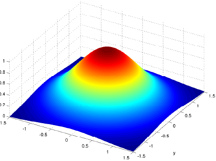
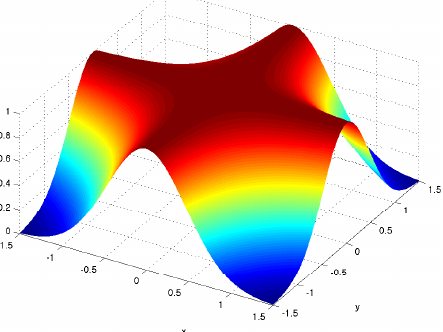
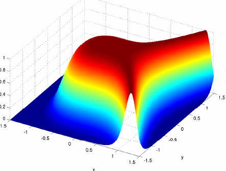
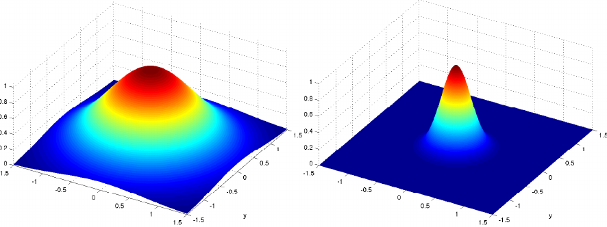
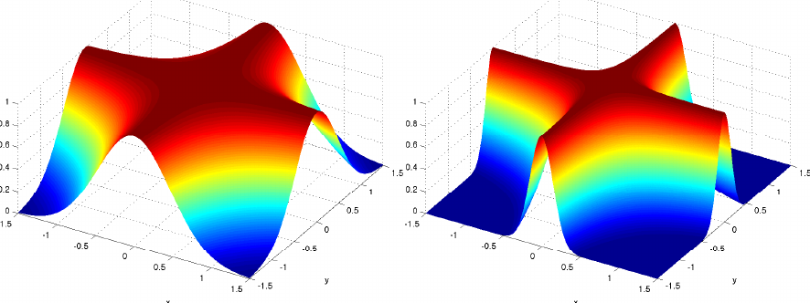
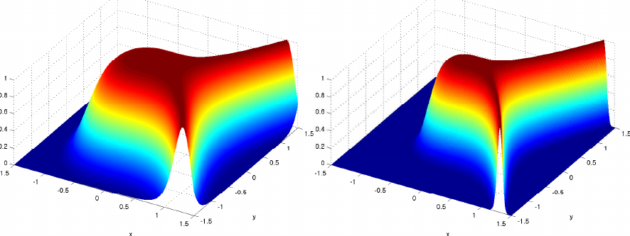
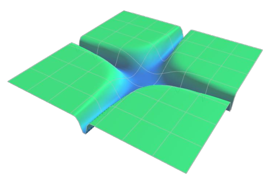
  • Parameters \(\omega = (x, y)\), data \(z\), true distribution \(q = p(\cdot|0, 0)\).
Regular. \(p(z|x, y) \propto e^{-(z_1-x)^2 - (z_2-y)^2}\), \(z \in \mathbb{R}^2\)
\(I(x, y) = x^2 + y^2\), \(\partial^2 I(0, 0) = \left(\begin{smallmatrix} 2 & 0 \\ 0 & 2 \end{smallmatrix}\right)\)
Singular. \(p(z|x, y) \propto e^{-(z - xy)^2}\), \(z \in \mathbb{R}\)
\(I(x, y) = (xy)^2\), \(\partial^2 I(0, 0) = 0\)
Singular. \(p(z|x, y) \propto e^{-(z - y^2 + x^3)^2}\), \(z \in \mathbb{R}\)
\(I(x, y) = (y^2 - x^3)^2\), \(\partial^2 I(0, 0) = 0\)

Singular Models Are Everywhere

  • Examples of singular models:
    • Layered neural networks
    • Normal mixtures, mixtures of statistical models
    • Reduced rank regressions
    • Boltzmann machines, Bayes networks
    • Hidden Markov models
    • Stochastic context-free grammars
  • Models with hierarchical structure or hidden variables are typically singular.

Breaking Classical Statistics

  • Singular models do not behave like regular models:
    • Maximum likelihood estimation is not efficient
    • The posterior is not asymptotically Gaussian
    • BIC: The Laplace approximation is incorrect
    • AIC: Generalization error is not proportional to \(d = \dim \Omega\)

Real Log Canonical Threshold (RLCT)

  • Let \(f(\omega)\) be a function with \(f(0)=0\). Let \(\Omega\) be a sufficiently small neighborhood of \(0\).
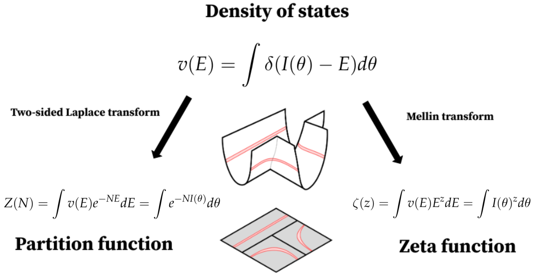
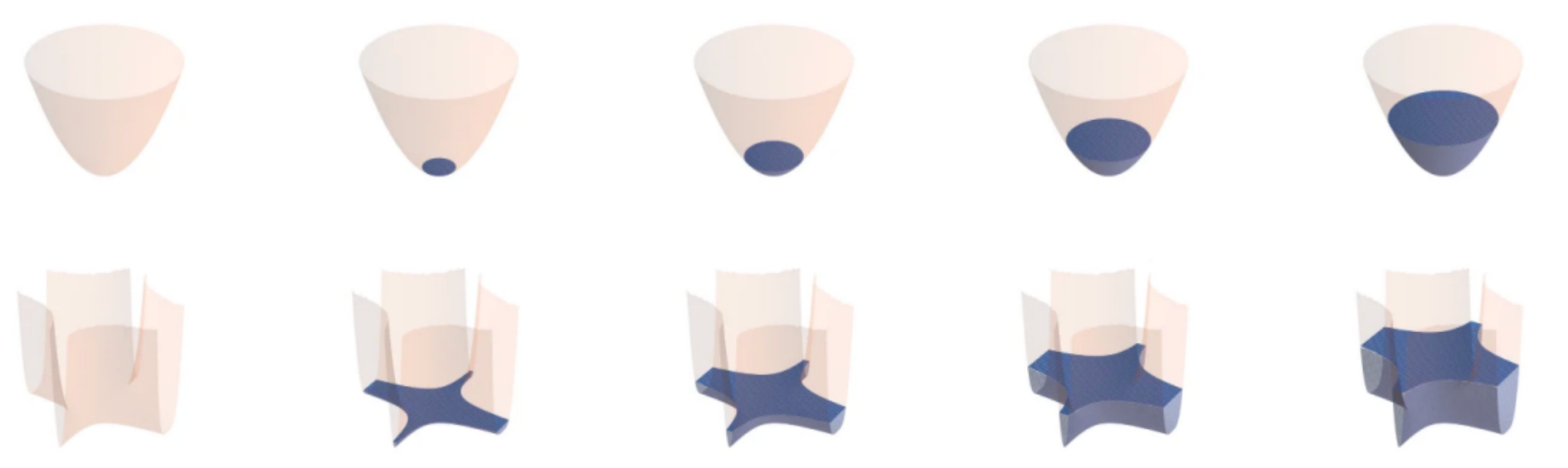
  • Asymptotically as \(\varepsilon \rightarrow 0\), the volume \(V(\varepsilon)\) of the tubular neighborhood approaches

\[ \begin{aligned} V(\varepsilon) &= \int_{\{\omega \in \Omega \,\mid\, f(\omega)<\varepsilon\}} d\omega \\ &\rightarrow C\varepsilon^\lambda (-\log \varepsilon)^{\theta-1}. \end{aligned} \]

  • Resolution of singularities implies that \(\lambda\) is a positive rational number (the real log canonical threshold at \(f\) at the origin), and \(\theta\) is a positive integer (its multiplicity).

RLCT Examples

Regular. \(f(x,y) = x^2 + y^2\)

\((\lambda, \theta) = (1, 1)\)
Singular. \(f(x,y) = (xy)^2\)

\((\lambda, \theta) = (\frac{1}{2}, 2)\)
Singular. \(f(x,y) = (y^2 - x^3)^2\)

\((\lambda, \theta) = (\frac{5}{12}, 1)\)

Algebraic Geometry

Resolution of Singularities

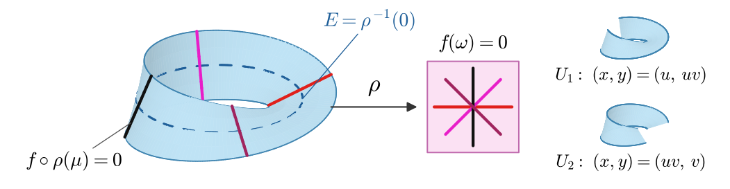
  • A resolution of singularities of \(f\) is a proper real analytic map \(\rho : U \rightarrow \Omega\), isomorphic over \(\{f \neq 0\}\), such that on each chart \(U_i\) of the manifold \(U\), \[ f \circ \rho(\mu) = a(\mu)\, \mu^{\kappa}, \qquad \det \partial\rho(\mu) = b(\mu)\, \mu^{\tau}, \] where \(a, b \neq 0\) on \(U_i\) and \(\mu^{\kappa} = \mu_1^{\kappa_1} \cdots \mu_d^{\kappa_d}\).
  • Theorem (Hironaka). Every real analytic function has a resolution of singularities.
The Learning Coefficient

  • The learning coefficient \(\lambda\) of a singular model at a parameter \(\omega_0\) with respect to the true distribution \(q\) is the RLCT of the relative information \(I(w) := I_{q\Vert p(\cdot \vert \omega)}(X)\) at \(\omega_0\).

  • The learning coefficient \(\lambda\) of a singular model over \(\Omega\) is the minimum of learning coefficients over all \(\omega \in \Omega\). Its multiplicity is the highest one available for \(\lambda\).

  • Regular models have \(\lambda = d/2\). Singular models have \(\lambda \leq d/2\).
Free Energy Formula

  • Theorem (Watanabe). If \(q\) is realizable, then the free energy or stochastic complexity has an asymptotic expansion (as \(n \rightarrow \infty\)) \[ F_n = n S_n + \lambda \log n - (\theta -1) \log \log n + O_p(1) \] where \(\lambda\) is the learning coefficient over \(\Omega\) with respect to \(q\), and \(\theta\) its multiplicity.

  • For regular models, \(\lambda = d/2\) and \(\theta = 1\). Since \(n L_n(\hat{\omega}) = n S_n + O_p(1)\) at the MLE \(\hat{\omega}\), this recovers the Bayesian Information Criterion \[ F_n = n L_n(\hat{\omega}) + \frac{d}{2} \log n + O_p(1). \]

Generalization Error Formula

  • Theorem (Watanabe). If \(q\) is realizable, then the expectation of the Bayes generalization error is asymptotically (as \(n \rightarrow \infty\)) \[ \mathbb{E}[G_n] = \frac{\lambda}{n} + o\left(\frac{1}{n}\right) \] where \(\lambda\) is the learning coefficient over \(\Omega\) with respect to \(q\).
  • For regular models, \(\lambda = d/2\), recovering the Akaike Information Criterion.

Deep Learning

Generalization: Classical Learning

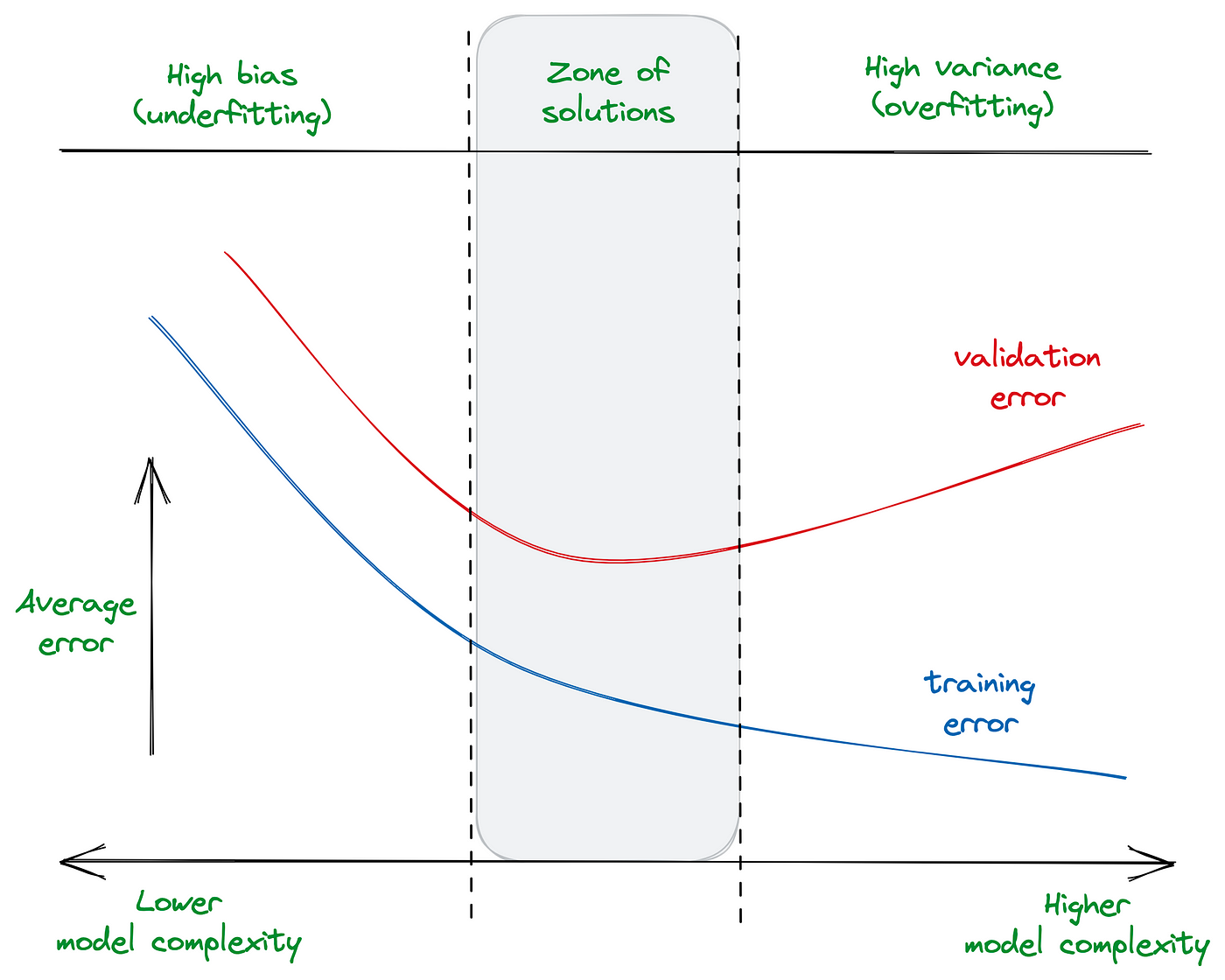
  • For regular models, maximum likelihood estimation overfits.
  • AIC and BIC deal with overfitting by penalizing the number of parameters: the BIC penalty is \(\frac{d}{2}\log n\)
    and the AIC penalty is \(\frac{d}{2}\).
  • These results do not apply to singular models such as deep neural nets.
Generalization: Deep Learning
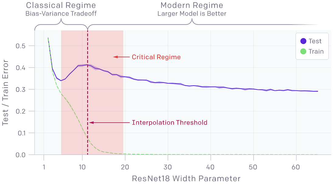
Double descent. Test error falls again as width grows past interpolation threshold.

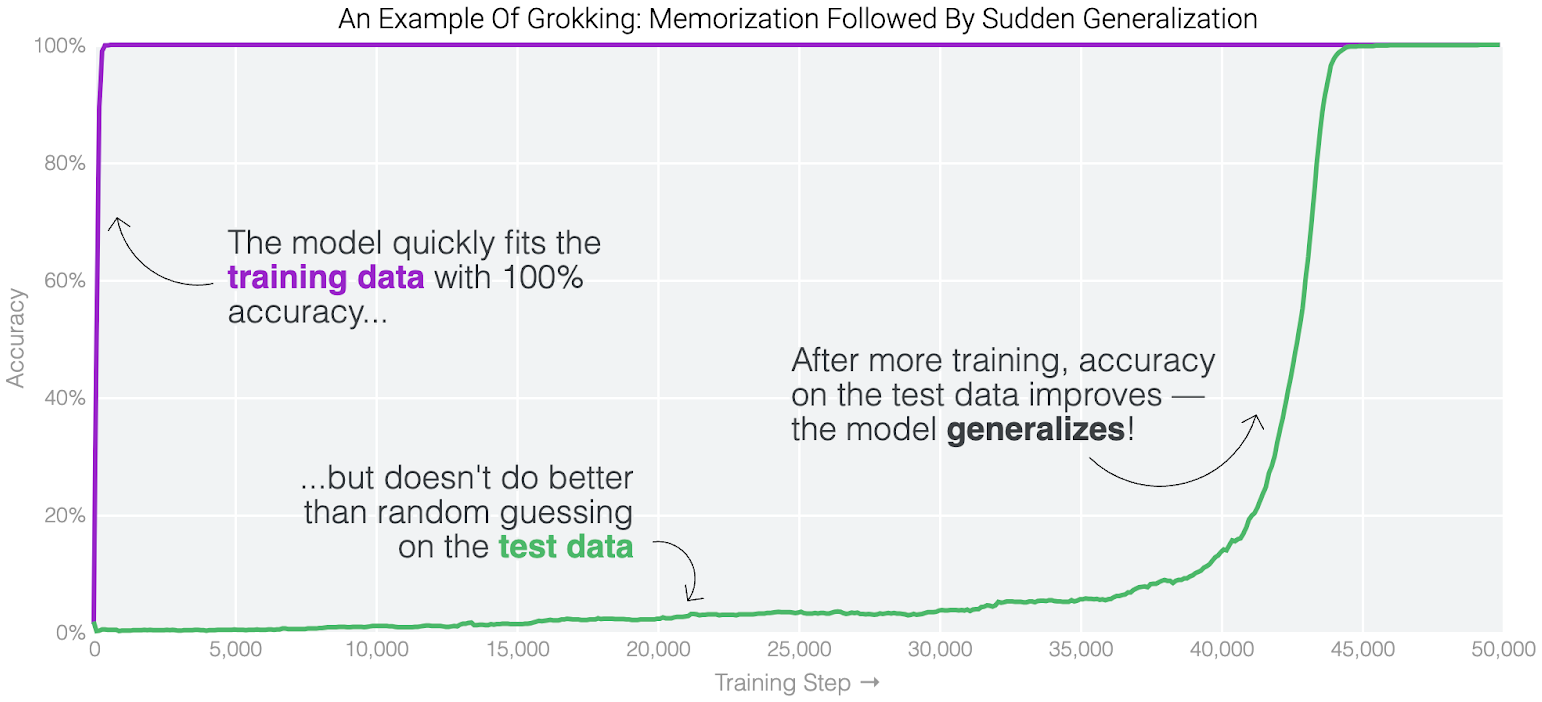
Grokking. Test accuracy jumps long after the training data is memorized.

Singularities in Deep Learning
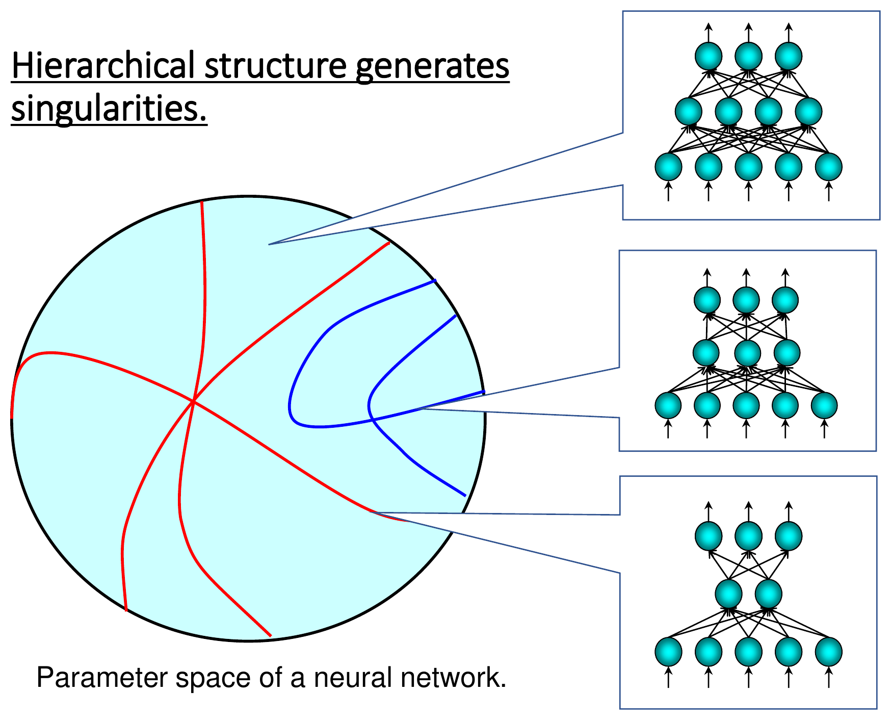
What Happens During Learning?
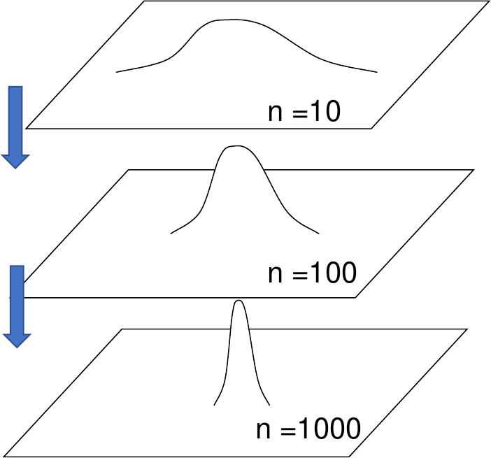
In regular models, the posterior concentrates on the best parameter as \(n\) grows: a gradual increase of confidence.
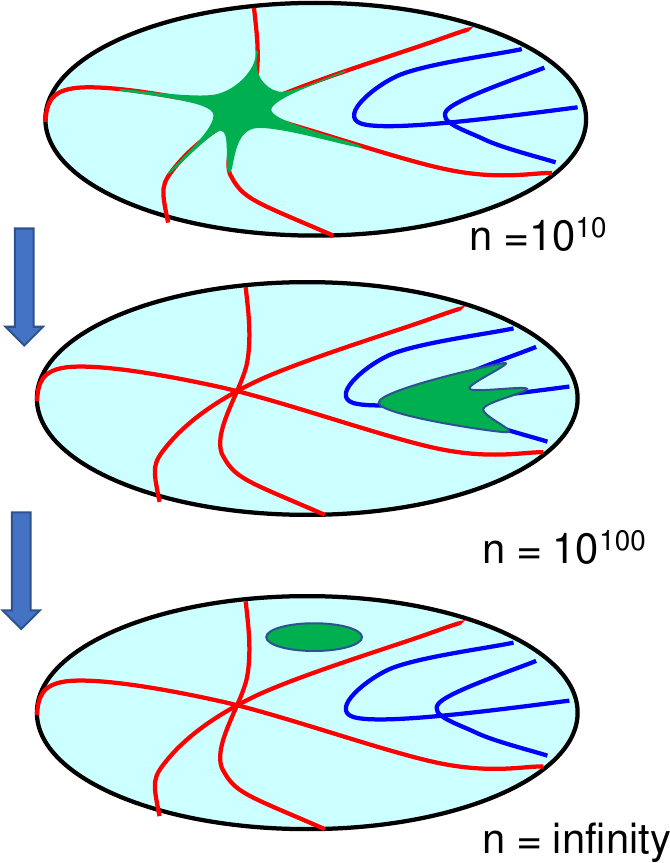
In singular models, the posterior jumps from one singularity to another. Even a huge \(n\) is far from infinity, so deep learning always remains in a singular state.

Internal Model Selection

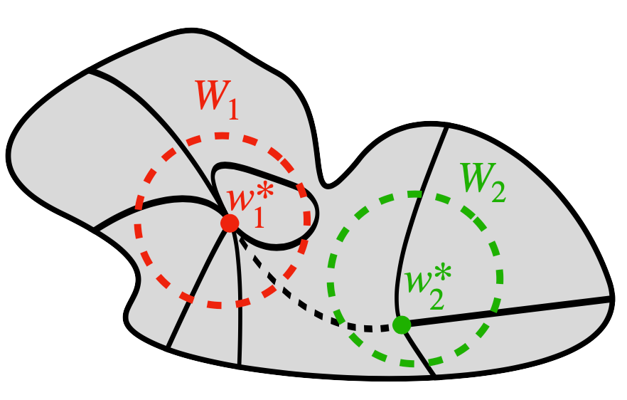
  • Suppose \(\Omega\) is partitioned into two subspaces \(W_1\) and \(W_2\). Then \[ \begin{align*} F_n(\Omega) &= -\log\big(e^{-F_n(W_1)} + e^{-F_n(W_2)}\big) \\ &\approx \min\{F_n(W_1), F_n(W_2)\}. \end{align*} \]
  • Restricting the free energy to a region \(W_\alpha \subset \Omega\) around a local minimum \(\omega^*_\alpha\), \[ F_n(W_\alpha) \approx n L_n(\omega^*_\alpha) + \lambda(\omega^*_\alpha) \log n. \]
  • Tradeoff between accuracy and complexity depends on the dataset size \(n\).
Free Energy Curves
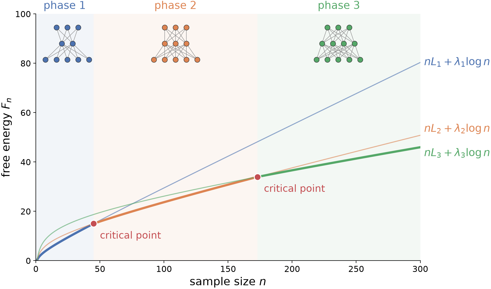
  • Each submodel has free energy \(nL_k + \lambda_k \log n\): smaller networks have larger loss \(L_k\) but smaller \(\lambda_k\). The full model has free energy \(F_n \approx \min_k \{nL_k + \lambda_k \log n\}\).
  • At each critical point, a more complex network takes over the minimum free energy, creating a phase transition.

Generalization Error Curves
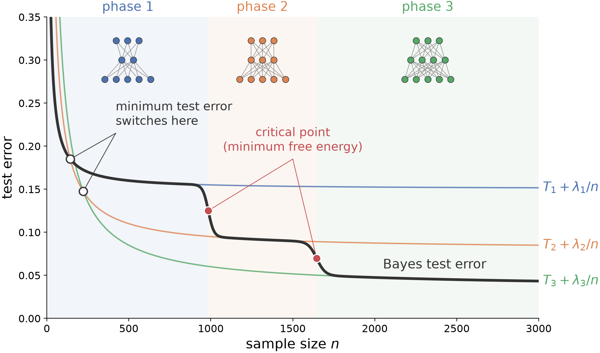
  • Each submodel has test error \(T_k + \lambda_k/n\), which is a proxy for the generalization error \(\mathbb{E}[G_n] \approx \lambda_k/n\).
  • The Bayes curve jumps at the free energy critical points (red), much later than where the test errors cross (white).

Local Posterior Sampling

  • Theorem (WBIC, Watanabe). At inverse temperature \(\beta^* = 1/\log n\), the posterior average of \(nL_n(\omega)\) estimates the free energy \(F_n\) to within \(O_p(\sqrt{\log n})\).
  • To measure the complexity of a trained network at \(\omega^*\), sample from the localized tempered posterior \[ p(\omega;\, \omega^*, \beta, \gamma) \;\propto\; \exp\Big( -n\beta\, L_n(\omega) - \frac{\gamma}{2}\,\Vert \omega - \omega^* \Vert^2 \Big). \]
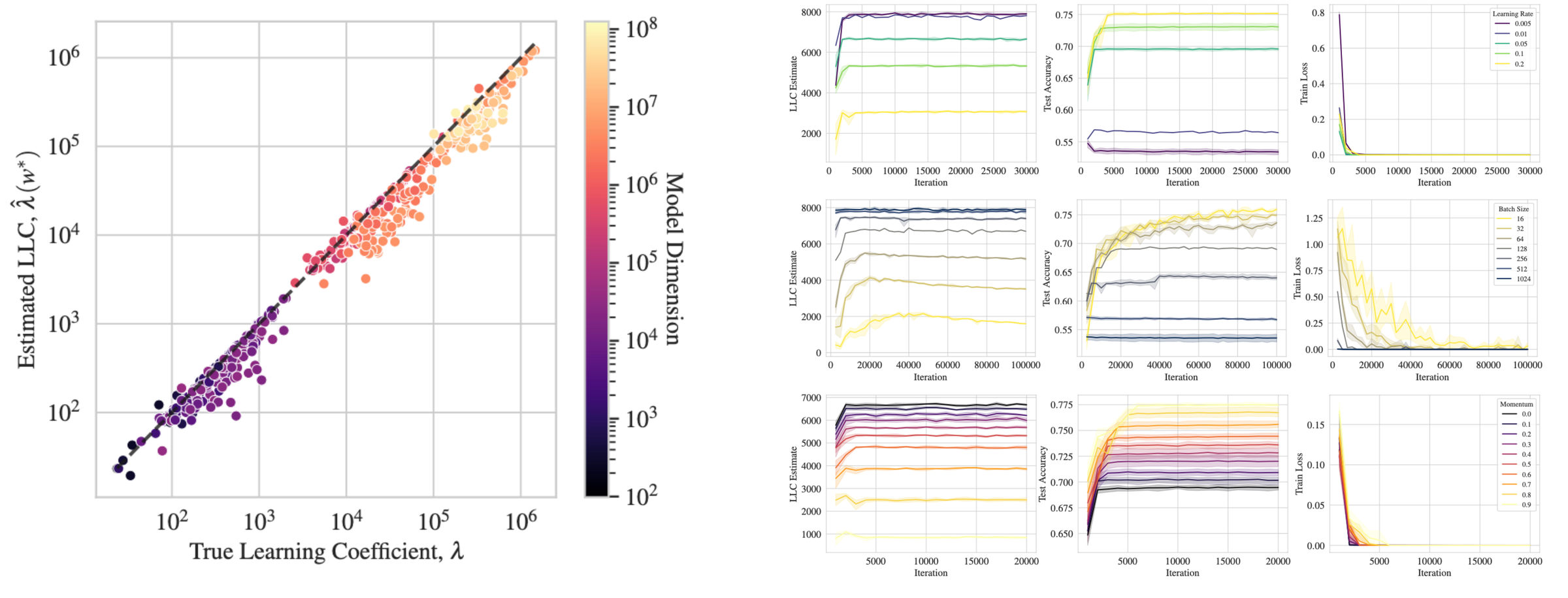
  • Local learning coefficient estimator: \[ \hat{\lambda}(\omega^*) = n\beta^* \Big( \mathbb{E}^{\beta^*}_{\omega^*,\gamma}\big[L_n(\omega)\big] - L_n(\omega^*) \Big). \]
  • Stochastic gradient Langevin dynamics (SGLD) on minibatches of size \(m\): \[ \Delta\omega_t = -\frac{\epsilon}{2}\Big( n\beta^*\, \nabla L_m(\omega_t) + \gamma(\omega_t - \omega^*) \Big) + \eta_t, \qquad \eta_t \sim \mathcal{N}(0, \epsilon I). \]

Estimating Learning Coefficients

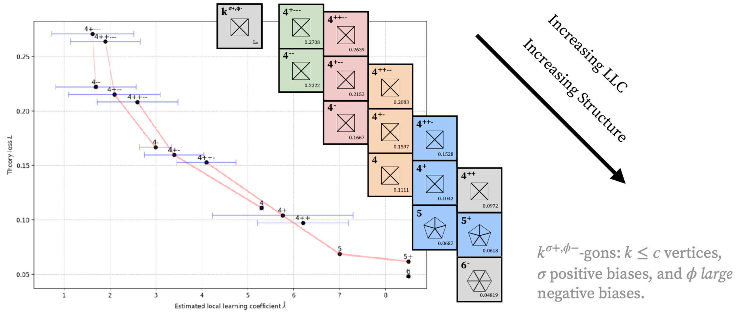
Toy Model of Superposition
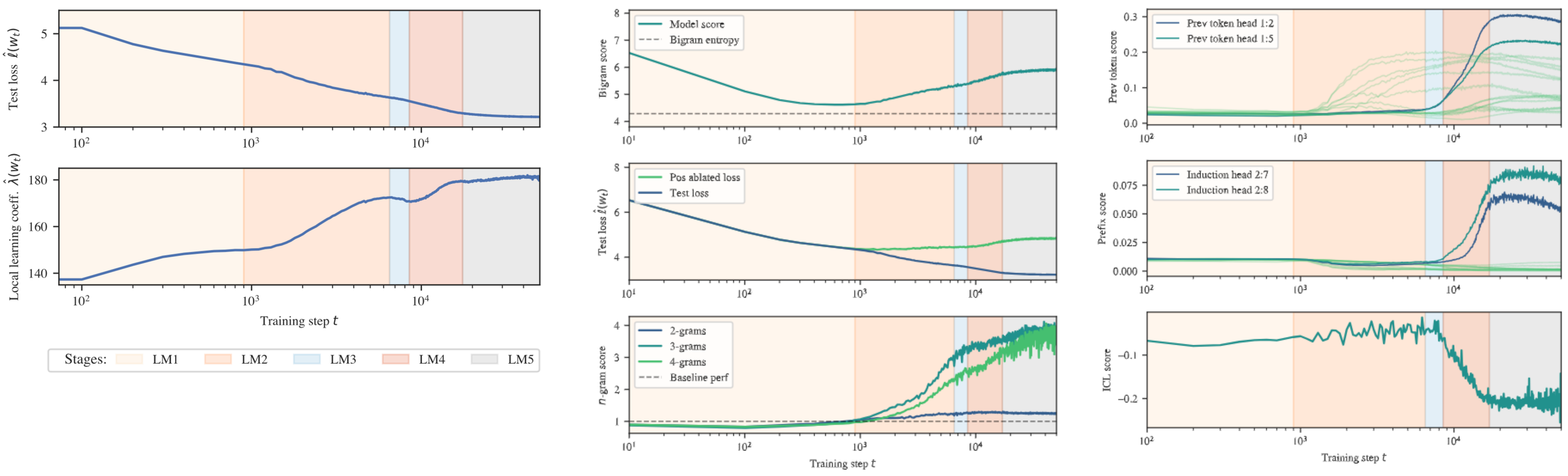
Stages of Language Models
Beyond Learning Coefficients
Deeper Theory?
More Resources

Thank you : )

https://shaoweilin.github.io/